Understanding Positional Encodings in Transformers

Part 1: The Position Problem & Sinusoidal Positional Encoding #

Why Transformers Need Help Knowing Where | A Six-Part Series

📚 Series Navigation:

• Part 1: The Position Problem & Sinusoidal PE ← You are here
• Part 2: Learned Positional Embeddings
• Part 3: RoPE (Rotary Position Embeddings) - Coming Soon
• Part 4: ALiBi (Attention with Linear Biases) - Coming Soon
• Part 5: PoPE (Polar Coordinate Embeddings) - Coming Soon
• Part 6: Practitioner's Guide - Coming Soon

Introduction #

Transformers have revolutionized natural language processing, computer vision, and many other domains. But there's a fundamental problem at their core: self-attention is permutation-invariant.

This means that without additional information, a transformer treats "The cat sat on the mat" identically to "mat the on sat cat The" — clearly problematic for understanding language!

This notebook explores:

1. Why transformers need positional information
2. How the original 2017 solution (sinusoidal positional encoding) works
3. The mathematical foundations and intuitions behind it
4. Visualizations to build deep understanding

📄 Paper: Attention Is All You Need (Vaswani et al., 2017)

1. Import Required Libraries #

First, let's import all the libraries we'll need. This notebook is fully self-contained.

# Install dependencies (run once)
!pip install -q numpy matplotlib seaborn torch plotly

# Core libraries
import numpy as np
import matplotlib.pyplot as plt
import seaborn as sns
import pandas as pd

# PyTorch
import torch
import torch.nn as nn
import torch.nn.functional as F
from typing import Optional, Tuple

# Interactive visualization
import plotly.graph_objects as go
import plotly.express as px

# Set visualization styles
sns.set_style('whitegrid')
plt.rcParams['figure.dpi'] = 100
plt.rcParams['figure.figsize'] = [10, 6]

# Set random seeds for reproducibility
np.random.seed(42)
torch.manual_seed(42)

print("✓ All libraries imported successfully!")
print(f"PyTorch version: {torch.__version__}")

✓ All libraries imported successfully!
PyTorch version: 2.9.1+cu128

2. The Permutation Invariance Problem #

Why Transformers Can't Tell Position #

Self-attention computes a weighted sum of all values, where weights depend only on the content of queries and keys — not their positions. Mathematically:

The problem: If we shuffle the input tokens, the attention scores change, but the set of outputs remains the same (just reordered). The model has no way to know which token came first, second, etc.

Let's demonstrate this with a simple example:

# Demonstrate permutation invariance
class SimpleAttentionNoPE(nn.Module):
    """Self-attention without any positional encoding"""
    def __init__(self, d_model: int, n_heads: int):
        super().__init__()
        self.attn = nn.MultiheadAttention(d_model, n_heads, batch_first=True)
    
    def forward(self, x):
        output, attn_weights = self.attn(x, x, x)
        return output, attn_weights

# Create a simple model
model = SimpleAttentionNoPE(d_model=32, n_heads=4)
model.eval()

# Create token embeddings (imagine these are words)
# "The cat sat on the mat" → 6 tokens
tokens_original = torch.randn(1, 6, 32)

# Permute the tokens (shuffle the word order)
permutation = torch.tensor([2, 0, 4, 1, 5, 3])  # Random shuffle
tokens_permuted = tokens_original[:, permutation, :]

with torch.no_grad():
    out_original, attn_original = model(tokens_original)
    out_permuted, attn_permuted = model(tokens_permuted)

# Check if outputs are just permutations of each other
# Unpermute the permuted output to compare
inverse_perm = torch.argsort(permutation)
out_permuted_reordered = out_permuted[:, inverse_perm, :]

difference = torch.abs(out_original - out_permuted_reordered).mean().item()

print("=" * 60)
print("PERMUTATION INVARIANCE DEMONSTRATION")
print("=" * 60)
print(f"\nOriginal token order:  [0, 1, 2, 3, 4, 5]")
print(f"Permuted token order:  {permutation.tolist()}")
print(f"\nMean difference after unpermuting: {difference:.8f}")
print("\n→ The outputs are nearly identical (just reordered)!")
print("→ The model CANNOT distinguish word order without PE!")

============================================================
PERMUTATION INVARIANCE DEMONSTRATION
============================================================

Original token order: [0, 1, 2, 3, 4, 5]
Permuted token order: [2, 0, 4, 1, 5, 3]

Mean difference after unpermuting: 0.00000002

→ The outputs are nearly identical (just reordered)!
→ The model CANNOT distinguish word order without PE!

Historical Context: How Did We Handle Position Before? #

RNNs and LSTMs (pre-2017):

• Processed tokens sequentially, one at a time
• Position was implicit in the hidden state evolution
• The 5th hidden state "remembered" it had seen 4 tokens before

Transformers (2017):

• Process all tokens in parallel for efficiency
• No sequential processing → no implicit position
• Solution: Explicitly inject position information via "positional encodings"

The challenge: How do we encode position in a way that:

1. Is unique for each position
2. Generalizes to different sequence lengths
3. Allows the model to learn relative positions
4. Doesn't interfere with semantic meaning

3. Sinusoidal Positional Encoding: The Original Solution #

The Key Insight #

Vaswani et al. (2017) proposed using sine and cosine functions at different frequencies to encode position. The intuition:

• Each dimension oscillates at a different rate
• Lower dimensions: high frequency (rapid oscillation)
• Higher dimensions: low frequency (slow oscillation)
• Together, they create a unique "fingerprint" for each position

Think of it like a clock with multiple hands moving at different speeds — at any moment, the combination of hand positions uniquely identifies the time.

Mathematical Formulation #

For position $\text{pos}$ and dimension $i$:

Where:

• $\text{pos}$: Position index (0, 1, 2, ...)
• $i$: Dimension pair index
• $d_{\text{model}}$: Total embedding dimension
• Even dimensions use sine, odd dimensions use cosine
• $10000$: Base that controls the wavelength range

def generate_sinusoidal_pe(seq_len: int, d_model: int) -> np.ndarray:
    """
    Generate sinusoidal positional encoding matrix.
    
    Args:
        seq_len: Maximum sequence length
        d_model: Dimension of the model (embedding size)
    
    Returns:
        Positional encoding matrix of shape (seq_len, d_model)
    """
    # Create position indices: [0, 1, 2, ..., seq_len-1]
    position = np.arange(seq_len)[:, np.newaxis]  # Shape: (seq_len, 1)
    
    # Create dimension indices for computing frequencies
    # We use pairs of dimensions, so we step by 2
    dim_indices = np.arange(0, d_model, 2)  # [0, 2, 4, ..., d_model-2]
    
    # Compute the division term: 10000^(2i/d_model)
    # This creates wavelengths from 2π to 10000*2π
    div_term = 10000 ** (dim_indices / d_model)  # Shape: (d_model/2,)
    
    # Initialize PE matrix
    pe = np.zeros((seq_len, d_model))
    
    # Apply sine to even indices
    pe[:, 0::2] = np.sin(position / div_term)
    
    # Apply cosine to odd indices
    pe[:, 1::2] = np.cos(position / div_term)
    
    return pe


# Generate positional encodings
d_model = 64
seq_len = 100

pe_matrix = generate_sinusoidal_pe(seq_len, d_model)

print(f"Generated positional encoding matrix: {pe_matrix.shape}")
print(f"  → {seq_len} positions × {d_model} dimensions")
print(f"Value range: [{pe_matrix.min():.3f}, {pe_matrix.max():.3f}]")
print("\n✓ Sinusoidal PE function implemented!")

Generated positional encoding matrix: (100, 64)
→ 100 positions × 64 dimensions
Value range: [-1.000, 1.000]

✓ Sinusoidal PE function implemented!

4. Visualizing the Positional Encoding Matrix #

Heatmap View #

Let's visualize the full positional encoding matrix. Each row is a position, each column is a dimension.

# Visualization 1: Full Heatmap
fig, ax = plt.subplots(figsize=(14, 8))

im = ax.imshow(pe_matrix, cmap='RdBu_r', aspect='auto', interpolation='nearest')
plt.colorbar(im, ax=ax, label='Encoding Value')

ax.set_xlabel('Dimension Index', fontsize=12)
ax.set_ylabel('Position Index', fontsize=12)
ax.set_title('Sinusoidal Positional Encoding\n(100 positions × 64 dimensions)', 
             fontsize=14, fontweight='bold')

# Add annotations for dimension types
ax.axhline(y=-0.5, color='black', linewidth=0.5)
ax.text(d_model//4, -3, 'High Frequency\n(local patterns)', ha='center', fontsize=10, color='blue')
ax.text(3*d_model//4, -3, 'Low Frequency\n(global patterns)', ha='center', fontsize=10, color='red')

plt.tight_layout()
plt.show()

print("Key observations:")
print("• Left side (low dimensions): Rapid oscillations — high frequency")
print("• Right side (high dimensions): Slow oscillations — low frequency")
print("• Each row (position) has a unique pattern across all dimensions")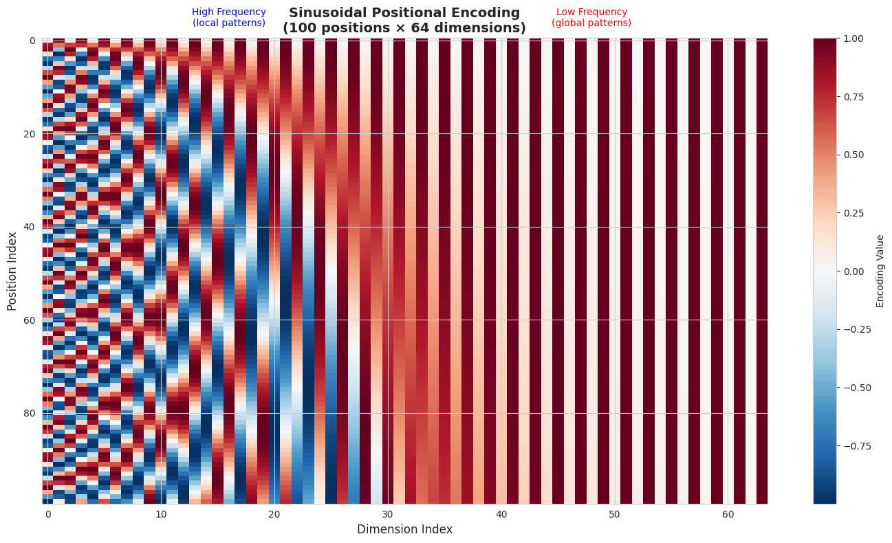

Key observations:
• Left side (low dimensions): Rapid oscillations — high frequency
• Right side (high dimensions): Slow oscillations — low frequency
• Each row (position) has a unique pattern across all dimensions

# Visualization 2: Detailed view of first 11 positions × 11 dimensions
pe_small = generate_sinusoidal_pe(11, 64)

fig, ax = plt.subplots(figsize=(13, 8))

sns.heatmap(pe_small[:, :11], 
            cmap='RdBu_r', 
            center=0, 
            ax=ax, 
            annot=True, 
            fmt='.2f',
            annot_kws={'size': 9},
            xticklabels=[f'Dim {i}' for i in range(11)],
            yticklabels=[f'Pos {i}' for i in range(11)],
            cbar_kws={'label': 'Encoding Value'})

ax.set_title('Detailed View: Positions 0-10 × Dimensions 0-10\n(d_model=64)', 
             fontsize=14, fontweight='bold', pad=20)
ax.set_xlabel('Dimension Index', fontsize=12)
ax.set_ylabel('Position Index', fontsize=12)

# Add sin/cos labels
for i in range(11):
    label = 'sin' if i % 2 == 0 else 'cos'
    color = 'blue' if i % 2 == 0 else 'red'
    ax.text(i + 0.5, -0.3, label, ha='center', va='top', fontsize=9, 
            color=color, fontweight='bold')

plt.tight_layout()
plt.show()

print("\nPattern Analysis:")
print("• Dim 0 (sin): Starts at 0.00, oscillates rapidly")
print("• Dim 1 (cos): Starts at 1.00, oscillates rapidly")
print("• Dim 10 (sin): Changes very slowly across positions")
print("• Each position has a unique combination of values!")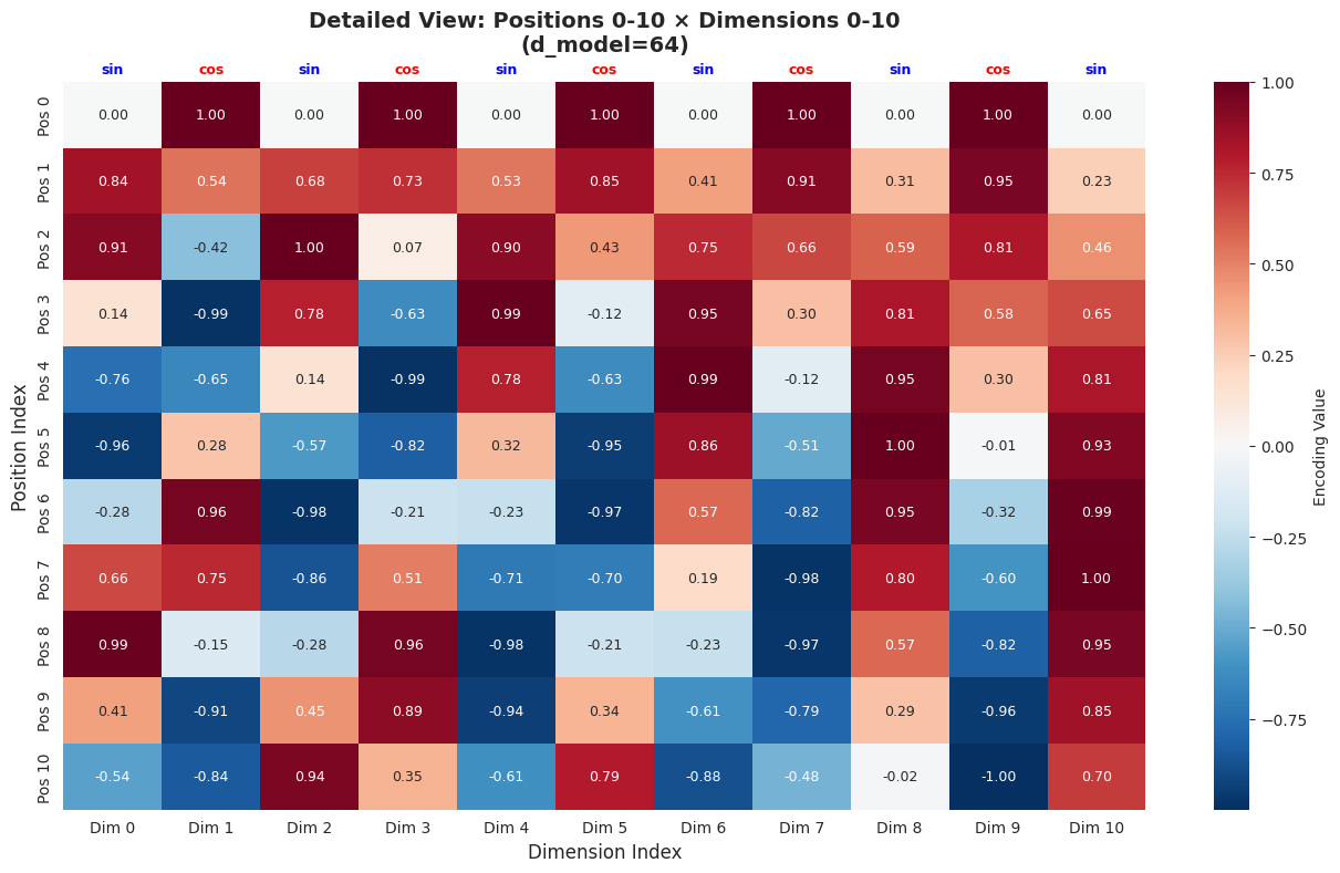

Pattern Analysis:
• Dim 0 (sin): Starts at 0.00, oscillates rapidly
• Dim 1 (cos): Starts at 1.00, oscillates rapidly
• Dim 10 (sin): Changes very slowly across positions
• Each position has a unique combination of values!

5. Individual Dimension Waves #

Let's plot the values for individual dimensions across positions to see the wave patterns clearly.

# Plot individual dimensions
dims_to_show = [0, 1, 2, 3, 10, 11, 30, 31, 62, 63]
positions = np.arange(100)

fig, axes = plt.subplots(2, 1, figsize=(14, 8), sharex=True)

# Sine dimensions (even)
ax1 = axes[0]
sine_dims = [d for d in dims_to_show if d % 2 == 0]
colors = plt.cm.viridis(np.linspace(0, 1, len(sine_dims)))
for dim, color in zip(sine_dims, colors):
    ax1.plot(positions, pe_matrix[:, dim], label=f'Dim {dim}', 
             linewidth=2, alpha=0.8, color=color)
ax1.set_ylabel('Encoding Value', fontsize=12)
ax1.set_title('SINE Dimensions (Even Indices)', fontsize=14, fontweight='bold')
ax1.legend(loc='upper right', ncol=3)
ax1.grid(True, alpha=0.3)
ax1.set_ylim(-1.1, 1.1)

# Cosine dimensions (odd)
ax2 = axes[1]
cosine_dims = [d for d in dims_to_show if d % 2 == 1]
colors = plt.cm.plasma(np.linspace(0, 1, len(cosine_dims)))
for dim, color in zip(cosine_dims, colors):
    ax2.plot(positions, pe_matrix[:, dim], label=f'Dim {dim}', 
             linewidth=2, alpha=0.8, color=color)
ax2.set_xlabel('Position', fontsize=12)
ax2.set_ylabel('Encoding Value', fontsize=12)
ax2.set_title('COSINE Dimensions (Odd Indices)', fontsize=14, fontweight='bold')
ax2.legend(loc='upper right', ncol=3)
ax2.grid(True, alpha=0.3)
ax2.set_ylim(-1.1, 1.1)

plt.tight_layout()
plt.show()

print("Key observations:")
print("• Dim 0-3 (low indices): Complete multiple oscillations over 100 positions")
print("• Dim 10-11 (mid indices): Slower oscillations")
print("• Dim 30-31 (high indices): Very slow change")
print("• Dim 62-63 (highest): Almost constant — encode very long-range patterns")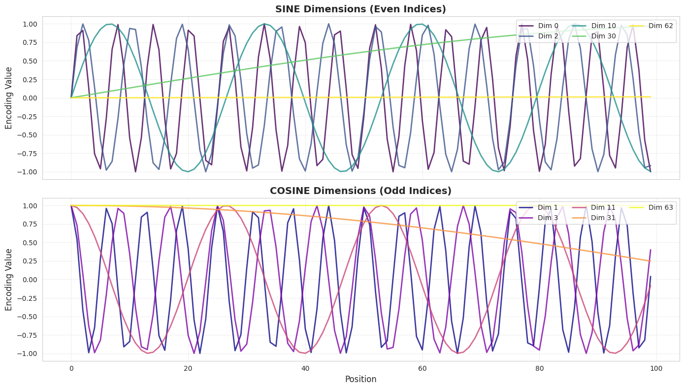

Key observations:
• Dim 0-3 (low indices): Complete multiple oscillations over 100 positions
• Dim 10-11 (mid indices): Slower oscillations
• Dim 30-31 (high indices): Very slow change
• Dim 62-63 (highest): Almost constant — encode very long-range patterns

6. Understanding the Wavelength Progression #

A critical insight: the wavelengths increase exponentially across dimensions. This creates a multi-scale encoding where different dimensions capture patterns at different ranges.

# Compute wavelengths for each dimension pair
def compute_wavelength(dim_pair: int, d_model: int) -> float:
    """Compute the wavelength (in position units) for a dimension pair"""
    return 2 * np.pi * (10000 ** (2 * dim_pair / d_model))

# Calculate wavelengths for all dimension pairs
dim_pairs = np.arange(d_model // 2)
wavelengths = [compute_wavelength(i, d_model) for i in dim_pairs]

# Visualization
fig, axes = plt.subplots(1, 2, figsize=(14, 5))

# Linear scale
ax1 = axes[0]
ax1.bar(dim_pairs * 2, wavelengths, color='steelblue', alpha=0.7)
ax1.set_xlabel('Dimension Index (even dimensions)', fontsize=12)
ax1.set_ylabel('Wavelength (position units)', fontsize=12)
ax1.set_title('Wavelength by Dimension (Linear Scale)', fontsize=14, fontweight='bold')
ax1.grid(True, alpha=0.3)

# Log scale
ax2 = axes[1]
ax2.bar(dim_pairs * 2, wavelengths, color='steelblue', alpha=0.7)
ax2.set_xlabel('Dimension Index (even dimensions)', fontsize=12)
ax2.set_ylabel('Wavelength (position units)', fontsize=12)
ax2.set_title('Wavelength by Dimension (Log Scale)', fontsize=14, fontweight='bold')
ax2.set_yscale('log')
ax2.grid(True, alpha=0.3, which='both')

plt.tight_layout()
plt.show()

# Print some specific wavelengths
print("Sample wavelengths:")
print(f"  Dimension 0:  {wavelengths[0]:.2f} positions (completes ~{100/wavelengths[0]:.1f} cycles in 100 positions)")
print(f"  Dimension 10: {wavelengths[5]:.2f} positions")
print(f"  Dimension 30: {wavelengths[15]:.2f} positions")
print(f"  Dimension 62: {wavelengths[31]:.2e} positions (extremely long wavelength)")
print("\n→ Exponential progression from ~6 positions to ~63,000 positions!")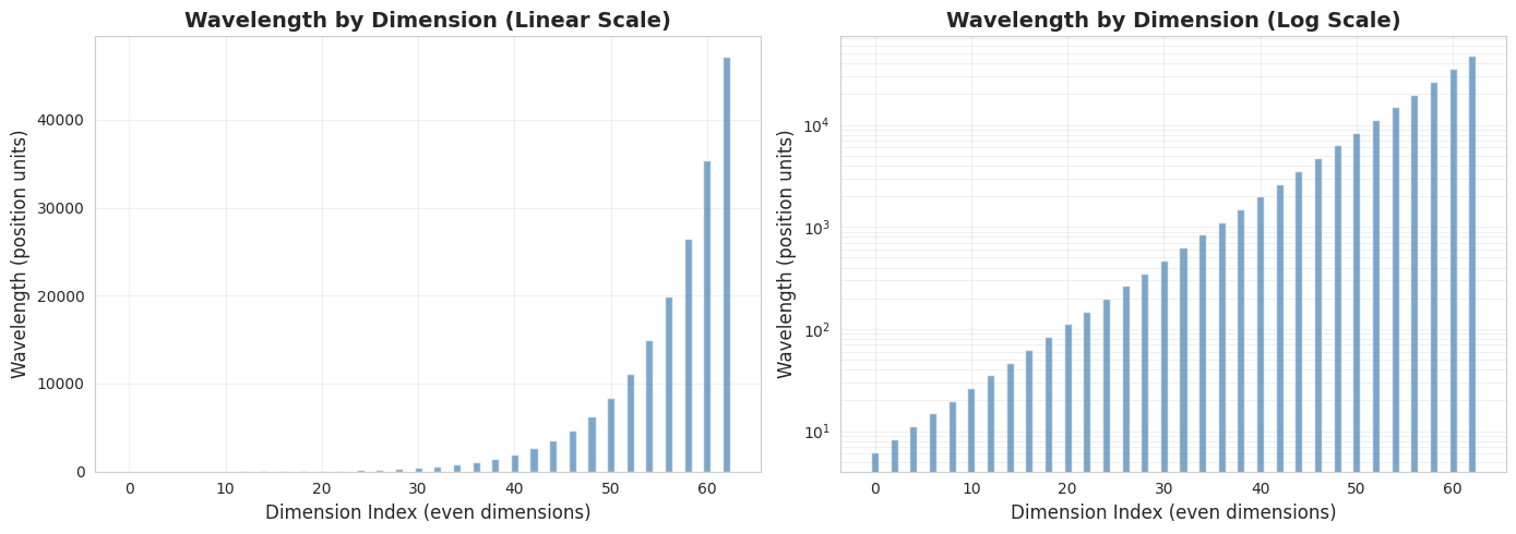

Sample wavelengths:
Dimension 0: 6.28 positions (completes ~15.9 cycles in 100 positions)
Dimension 10: 26.50 positions
Dimension 30: 471.17 positions
Dimension 62: 4.71e+04 positions (extremely long wavelength)

→ Exponential progression from ~6 positions to ~63,000 positions!

7. PyTorch Implementation: Sinusoidal PE Module #

Now let's implement a proper PyTorch module that can be used in a transformer.

class SinusoidalPositionalEncoding(nn.Module):
    """
    Sinusoidal positional encoding module for transformers.
    
    This module adds fixed sinusoidal positional encodings to input embeddings,
    following the original "Attention Is All You Need" paper (Vaswani et al., 2017).
    
    Args:
        d_model: Dimension of the model embeddings
        max_len: Maximum sequence length to precompute
        dropout: Dropout probability applied after adding PE
    """
    
    def __init__(self, d_model: int, max_len: int = 5000, dropout: float = 0.1):
        super().__init__()
        self.dropout = nn.Dropout(p=dropout)
        
        # Create positional encoding matrix
        pe = torch.zeros(max_len, d_model)
        
        # Position indices: [0, 1, 2, ..., max_len-1]
        position = torch.arange(0, max_len, dtype=torch.float).unsqueeze(1)
        
        # Compute division term for frequencies
        # exp(arange * -log(10000) / d_model) = 10000^(-arange/d_model)
        div_term = torch.exp(
            torch.arange(0, d_model, 2).float() * (-np.log(10000.0) / d_model)
        )
        
        # Apply sine to even indices
        pe[:, 0::2] = torch.sin(position * div_term)
        # Apply cosine to odd indices
        pe[:, 1::2] = torch.cos(position * div_term)
        
        # Add batch dimension: (1, max_len, d_model)
        pe = pe.unsqueeze(0)
        
        # Register as buffer (saved with model, but not a parameter)
        self.register_buffer('pe', pe)
    
    def forward(self, x: torch.Tensor) -> torch.Tensor:
        """
        Add positional encoding to input embeddings.
        
        Args:
            x: Input tensor of shape (batch_size, seq_len, d_model)
        
        Returns:
            Tensor with positional encoding added, same shape as input
        """
        # Add positional encoding (broadcasts across batch)
        x = x + self.pe[:, :x.size(1), :]
        return self.dropout(x)


# Test the module
batch_size = 2
seq_len = 10
d_model = 64

pos_encoder = SinusoidalPositionalEncoding(d_model)

# Create dummy input (simulating token embeddings)
x = torch.randn(batch_size, seq_len, d_model)

# Apply positional encoding
output = pos_encoder(x)

print(f"Input shape:  {x.shape}")
print(f"Output shape: {output.shape}")
print(f"PE buffer shape: {pos_encoder.pe.shape}")
print(f"\n✓ SinusoidalPositionalEncoding module working!")

Input shape: torch.Size([2, 10, 64])
Output shape: torch.Size([2, 10, 64])
PE buffer shape: torch.Size([1, 5000, 64])

✓ SinusoidalPositionalEncoding module working!

8. A Simple Transformer Layer with Positional Encoding #

Let's combine our positional encoding with self-attention to build a simple transformer layer.

class SimpleTransformerLayer(nn.Module):
    """
    A simple transformer layer demonstrating positional encoding usage.
    
    Components:
    1. Positional encoding (added to input)
    2. Multi-head self-attention
    3. Layer normalization with residual connection
    """
    
    def __init__(self, d_model: int, n_heads: int, dropout: float = 0.1):
        super().__init__()
        self.pos_encoding = SinusoidalPositionalEncoding(d_model, dropout=dropout)
        self.self_attn = nn.MultiheadAttention(
            d_model, n_heads, dropout=dropout, batch_first=True
        )
        self.norm = nn.LayerNorm(d_model)
        
    def forward(self, x: torch.Tensor) -> Tuple[torch.Tensor, torch.Tensor]:
        """
        Forward pass through the transformer layer.
        
        Args:
            x: Input tensor of shape (batch_size, seq_len, d_model)
        
        Returns:
            output: Transformed tensor, same shape as input
            attn_weights: Attention weight matrix (batch, seq_len, seq_len)
        """
        # Add positional encoding
        x_pos = self.pos_encoding(x)
        
        # Self-attention
        attn_output, attn_weights = self.self_attn(x_pos, x_pos, x_pos)
        
        # Residual connection and normalization
        output = self.norm(x + attn_output)
        
        return output, attn_weights


# Create and test the layer
layer = SimpleTransformerLayer(d_model=64, n_heads=8)
x = torch.randn(2, 20, 64)  # (batch, seq_len, d_model)

output, attn_weights = layer(x)

print(f"Input shape: {x.shape}")
print(f"Output shape: {output.shape}")
print(f"Attention weights shape: {attn_weights.shape}")
print("\n✓ Transformer layer with positional encoding working!")

Input shape: torch.Size([2, 20, 64])
Output shape: torch.Size([2, 20, 64])
Attention weights shape: torch.Size([2, 20, 20])

✓ Transformer layer with positional encoding working!

9. Visualizing Attention Patterns #

Let's look at how the attention weights are distributed. With positional encoding, we expect the model to develop position-aware attention patterns.

# Visualize attention patterns
fig, ax = plt.subplots(figsize=(10, 8))

# Get attention weights from first sample
attn_matrix = attn_weights[0].detach().numpy()

sns.heatmap(attn_matrix, 
            cmap='YlOrRd', 
            ax=ax, 
            square=True,
            cbar_kws={'label': 'Attention Weight'},
            xticklabels=5,
            yticklabels=5)

ax.set_xlabel('Key Position (attended to)', fontsize=12)
ax.set_ylabel('Query Position (attending from)', fontsize=12)
ax.set_title('Self-Attention Pattern\n(with Sinusoidal Positional Encoding)', 
             fontsize=14, fontweight='bold')

plt.tight_layout()
plt.show()

print("The attention pattern shows how each position (row) attends to other positions (columns).")
print("With PE, the model can learn position-dependent attention patterns.")
print("\nNote: This is a randomly initialized model — trained models show more structured patterns.")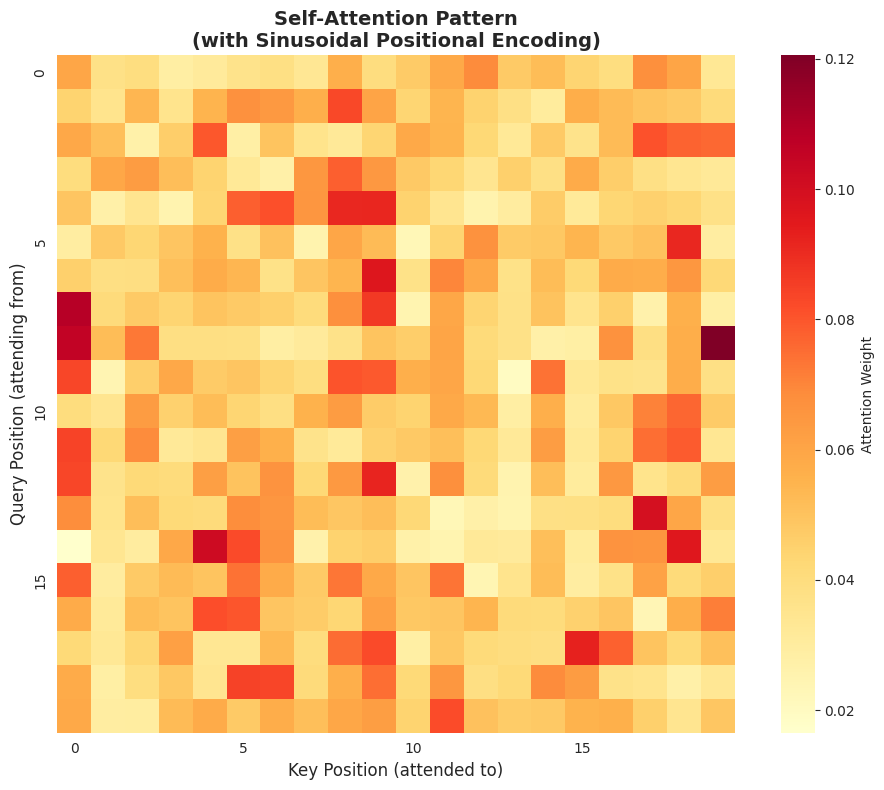

The attention pattern shows how each position (row) attends to other positions (columns).
With PE, the model can learn position-dependent attention patterns.

Note: This is a randomly initialized model — trained models show more structured patterns.

10. The Critical Question: Does PE Contaminate Token Meaning? #

You might wonder: by adding positional encoding directly to token embeddings, aren't we "contaminating" the semantic meaning of words?

Yes, we are mixing signals — and this is a known limitation!

Let's analyze the magnitude of this mixing:

# Analyze the mixing of token and positional information
token_emb = torch.randn(1, 128) * 0.5  # Typical embedding initialization scale
pos_enc = torch.tensor(generate_sinusoidal_pe(1, 128), dtype=torch.float32)

# Compute norms
token_norm = torch.norm(token_emb).item()
pos_norm = torch.norm(pos_enc).item()
combined = token_emb + pos_enc
combined_norm = torch.norm(combined).item()

# Compute angle between original and combined
dot_product = torch.dot(token_emb.flatten().float(), combined.flatten().float()).item()
cos_angle = dot_product / (token_norm * combined_norm)
angle_degrees = np.degrees(np.arccos(np.clip(cos_angle, -1, 1)))

print("=" * 60)
print("MAGNITUDE ANALYSIS: Token vs Positional Encoding")
print("=" * 60)
print(f"\nToken embedding norm:     {token_norm:.4f}")
print(f"Positional encoding norm: {pos_norm:.4f}")
print(f"Combined norm:            {combined_norm:.4f}")
print(f"\nAngle between original token emb and combined: {angle_degrees:.2f}°")
print("  (0° = identical direction, 90° = orthogonal)")

# Visualize
fig, ax = plt.subplots(figsize=(12, 4))
dims_to_show = 20
x_pos = np.arange(dims_to_show)
width = 0.25

ax.bar(x_pos - width, token_emb[0, :dims_to_show].numpy(), width, 
       label='Token Embedding', alpha=0.7, color='blue')
ax.bar(x_pos, pos_enc[0, :dims_to_show].numpy(), width, 
       label='Positional Encoding', alpha=0.7, color='orange')
ax.bar(x_pos + width, combined[0, :dims_to_show].numpy(), width, 
       label='Combined', alpha=0.7, color='green')

ax.set_xlabel('Dimension Index', fontsize=12)
ax.set_ylabel('Value', fontsize=12)
ax.set_title('Token Embedding + Positional Encoding (First 20 Dimensions)', 
             fontsize=14, fontweight='bold')
ax.legend()
ax.grid(True, alpha=0.3)

plt.tight_layout()
plt.show()

print("\n" + "=" * 60)
print("WHY IT STILL WORKS:")
print("=" * 60)
print("1. High-dimensional space has room for both signals")
print("2. The model learns to disentangle during training")
print("3. PE values are bounded in [-1, 1]")
print("\nBUT: Modern methods (RoPE, ALiBi, PoPE) address this better!")
print("     → See Parts 3, 4, and 5 of this series")

============================================================
MAGNITUDE ANALYSIS: Token vs Positional Encoding
============================================================

Token embedding norm: 5.5801
Positional encoding norm: 8.0000
Combined norm: 10.1047

Angle between original token emb and combined: 52.12°
(0° = identical direction, 90° = orthogonal)

============================================================
WHY IT STILL WORKS:
============================================================
1. High-dimensional space has room for both signals
2. The model learns to disentangle during training
3. PE values are bounded in [-1, 1]

BUT: Modern methods (RoPE, ALiBi, PoPE) address this better!
→ See Parts 3, 4, and 5 of this series

11. Properties of Sinusoidal Positional Encoding #

Let's verify some key mathematical properties that make sinusoidal PE effective.

Property 1: Bounded Values #

All PE values are in [-1, 1], preventing gradient explosion.

# Property 1: Bounded values
pe_long = generate_sinusoidal_pe(10000, 512)
print("Property 1: Bounded Values")
print(f"  PE matrix shape: {pe_long.shape}")
print(f"  Min value: {pe_long.min():.6f}")
print(f"  Max value: {pe_long.max():.6f}")
print("  ✓ All values in [-1, 1] as expected from sin/cos")

# Property 2: Unique positions
print("\nProperty 2: Unique Positions")
# Check if any two positions have identical encodings
n_positions = 1000
pe_check = generate_sinusoidal_pe(n_positions, 64)
unique_rows = len(np.unique(pe_check, axis=0))
print(f"  Checking {n_positions} positions...")
print(f"  Unique encoding vectors: {unique_rows}")
print(f"  ✓ Each position has a unique encoding")

# Property 3: Relative position via dot product
print("\nProperty 3: Relative Position Awareness")
# Dot products should decrease as distance increases
pos_0 = pe_check[0]
distances = [1, 2, 5, 10, 20, 50]
dot_products = [np.dot(pos_0, pe_check[d]) for d in distances]

fig, ax = plt.subplots(figsize=(10, 5))
ax.plot(distances, dot_products, 'o-', linewidth=2, markersize=8)
ax.set_xlabel('Distance from Position 0', fontsize=12)
ax.set_ylabel('Dot Product with Position 0', fontsize=12)
ax.set_title('Dot Product vs Distance (Demonstrates Relative Position Encoding)', 
             fontsize=14, fontweight='bold')
ax.grid(True, alpha=0.3)
plt.tight_layout()
plt.show()

print("  Dot product decreases with distance, encoding relative position!")

Property 1: Bounded Values
PE matrix shape: (10000, 512)
Min value: -1.000000
Max value: 1.000000
✓ All values in [-1, 1] as expected from sin/cos

Property 2: Unique Positions
Checking 1000 positions...
Unique encoding vectors: 1000
✓ Each position has a unique encoding

Property 3: Relative Position Awareness

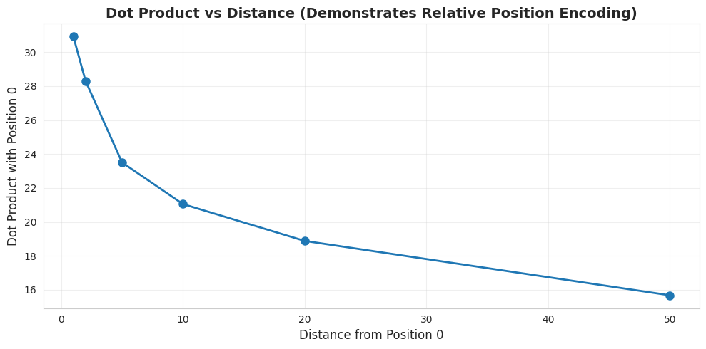
Dot product decreases with distance, encoding relative position!

12. The Relative Position Property #

One of the most elegant aspects of sinusoidal PE is that relative positions can be expressed as linear transformations. Due to trigonometric identities:

This means that $PE_{pos+k}$ can be expressed as a linear function of $PE_{pos}$!

# Demonstrate the linear transformation property
def relative_position_matrix(k: int, d_model: int) -> np.ndarray:
    """
    Compute the matrix M_k such that PE[pos+k] ≈ M_k @ PE[pos]
    for each dimension pair.
    
    For a sin/cos pair with frequency omega:
    [sin((pos+k)*omega)]   [cos(k*omega)   sin(k*omega)] [sin(pos*omega)]
    [cos((pos+k)*omega)] = [-sin(k*omega)  cos(k*omega)] [cos(pos*omega)]
    """
    # For each pair of dimensions, create a 2x2 rotation matrix
    n_pairs = d_model // 2
    M = np.zeros((d_model, d_model))
    
    for i in range(n_pairs):
        omega = 1.0 / (10000 ** (2 * i / d_model))
        angle = k * omega
        
        # Rotation matrix for this pair
        cos_k = np.cos(angle)
        sin_k = np.sin(angle)
        
        # Place in the big matrix (dimensions 2i and 2i+1)
        M[2*i, 2*i] = cos_k
        M[2*i, 2*i+1] = sin_k
        M[2*i+1, 2*i] = -sin_k
        M[2*i+1, 2*i+1] = cos_k
    
    return M


# Test: Can we predict PE[pos+k] from PE[pos] using a linear transform?
d_test = 64
pe_test = generate_sinusoidal_pe(100, d_test)

# For offset k=5, predict PE[10] from PE[5]
k = 5
M_k = relative_position_matrix(k, d_test)

pe_5 = pe_test[5]
pe_10_predicted = M_k @ pe_5
pe_10_actual = pe_test[10]

error = np.linalg.norm(pe_10_predicted - pe_10_actual)

print("Testing: Can PE[pos+k] be computed from PE[pos] via linear transform?")
print(f"\nOffset k = {k}")
print(f"Predicting PE[10] from PE[5]...")
print(f"Prediction error: {error:.2e}")
print("✓ Near-zero error confirms the linear transformation property!")

# Visualize
fig, axes = plt.subplots(1, 3, figsize=(15, 4))

axes[0].plot(pe_5[:20], 'o-', label='PE[5]')
axes[0].set_title('PE at Position 5', fontweight='bold')
axes[0].set_xlabel('Dimension')
axes[0].grid(True, alpha=0.3)

axes[1].plot(pe_10_actual[:20], 'o-', label='Actual', color='green')
axes[1].plot(pe_10_predicted[:20], 'x--', label='Predicted', color='red', alpha=0.7)
axes[1].set_title('PE at Position 10: Actual vs Predicted', fontweight='bold')
axes[1].set_xlabel('Dimension')
axes[1].legend()
axes[1].grid(True, alpha=0.3)

# Show the transformation matrix structure
axes[2].imshow(M_k[:16, :16], cmap='RdBu_r', aspect='equal')
axes[2].set_title(f'Transformation Matrix M_{k} (16×16 corner)', fontweight='bold')
axes[2].set_xlabel('Input Dimension')
axes[2].set_ylabel('Output Dimension')

plt.tight_layout()
plt.show()

print("\nThe block-diagonal structure shows 2×2 rotation matrices for each dimension pair.")

Testing: Can PE[pos+k] be computed from PE[pos] via linear transform?

Offset k = 5
Predicting PE[10] from PE[5]...
Prediction error: 5.14e-16
✓ Near-zero error confirms the linear transformation property!

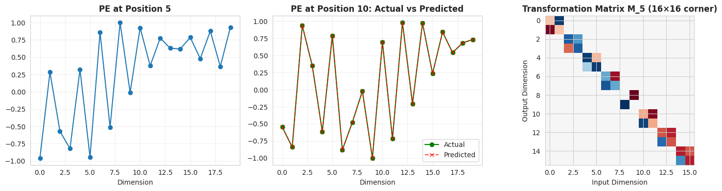
The block-diagonal structure shows 2×2 rotation matrices for each dimension pair.

13. Limitations of Sinusoidal PE #

While sinusoidal PE was groundbreaking in 2017, it has several limitations that motivated later improvements:

Limitation 1: Mixing of Semantic and Positional Information #

As we saw earlier, adding PE to token embeddings mixes the signals.

Limitation 2: Relative Position is Implicit #

The model must learn to extract relative positions from the combined embedding. RoPE (Part 3) makes this explicit.

Limitation 3: Fixed Encoding #

The encoding is deterministic and cannot adapt to task-specific positional patterns. Learned embeddings (Part 2) address this.

Limitation 4: No Causal Structure #

The same PE is used for all attention patterns. ALiBi (Part 4) introduces explicit distance penalties.

14. Summary and Key Takeaways #

What We Learned #

1. The Position Problem: Transformers are permutation-invariant without PE

   • Self-attention treats input as an unordered set
   • Word order is lost without explicit position information

2. Sinusoidal PE Solution (Vaswani et al., 2017):

   • Uses sine and cosine functions at different frequencies
   • Lower dimensions: high frequency (local patterns)
   • Higher dimensions: low frequency (global patterns)
   • Creates unique "fingerprint" for each position

3. Mathematical Formula:
   

   $$PE_{(pos, 2i)} = \sin\left(\frac{pos}{10000^{2i/d}}\right)$$
   
   
   $$PE_{(pos, 2i+1)} = \cos\left(\frac{pos}{10000^{2i/d}}\right)$$

4. Key Properties:

   • Bounded values [-1, 1]
   • Unique encoding for each position
   • Relative positions expressible as linear transforms

5. Limitations:

   • Mixes semantic and positional information
   • Relative position is implicit, not explicit
   • Cannot adapt to task-specific patterns

Coming Up Next #

Part 2: Learned Positional Embeddings

• The BERT/GPT-2 approach: just learn the positions!
• Trade-offs between fixed and learned encodings
• The extrapolation problem

References #

1. Vaswani, A., et al. (2017). "Attention Is All You Need." NeurIPS.

   • arxiv.org/abs/1706.03762
   • The original transformer paper introducing sinusoidal PE

2. Shaw, P., et al. (2018). "Self-Attention with Relative Position Representations." NAACL.

   • arxiv.org/abs/1803.02155
   • Early work on explicit relative position encoding

Last updated: January 2026

• Next: Learning Position — Trainable Embeddings from BERT to GPT
• Previous: Claude Code Power Tips