Multimodal search in 200 lines — EmbeddingGemma 2
by John Robinson @johnrobinsn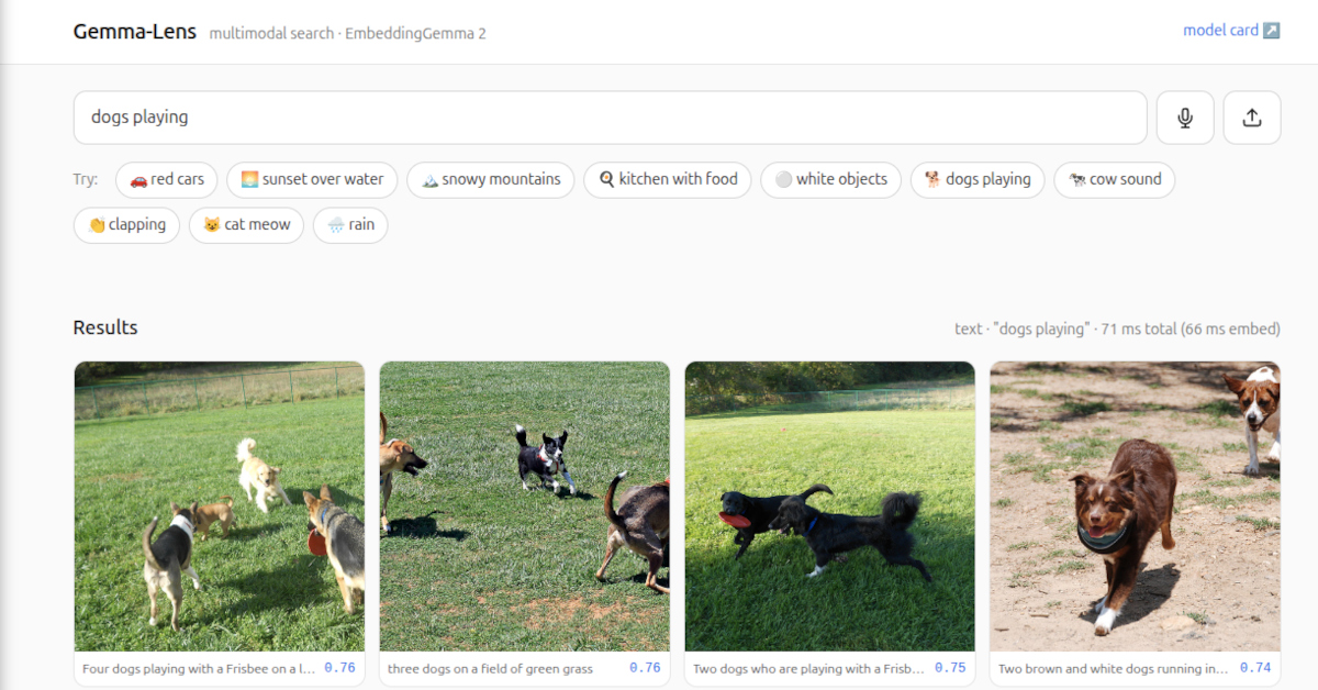
TL;DR — Google DeepMind released EmbeddingGemma 2 on 2026-10-06 — one 740M model that embeds text, images, and audio into the same 768-dimensional space. I used it to build Gemma-Lens, a working multimodal search engine over 5,000 COCO images + 2,000 ESC-50 audio clips. You type "cow mooing" and get cow sounds. You click a mic button and moo at your phone and get cow images. The point of this piece is to walk you through how a modern multimodal search engine actually works end-to-end, in code you can read in one sitting — not to benchmark the model to its limits. The latency numbers that show up later (~50 ms text query, ~125 ms audio query on an RTX 5090) are a happy side effect of the model being small and the stack being deliberately simple. Repo: https://github.com/johnrobinsn/gemma-lens.
This article is paired with a public code repo at https://github.com/johnrobinsn/gemma-lens — together they give you a reproducible recipe: one uv sync to install, one python -m gemma_lens.ingest to build the search index (one-time, ~7 min on a modern GPU), one uv run gemma-lens to serve, and you have a localhost multimodal search engine with a mic button and an upload button that answers queries in ~50 ms. No GPU? It still works on CPU — slower, but a modern laptop handles text queries in ~60-90 ms. Gemma-Lens is written for clarity, not for throughput. It is a reference implementation — a thing you can read top to bottom to build an accurate mental model of how a multimodal retrieval stack fits together. There is no serving layer, no batching, no CUDA-graph warmup, no quantization. Every one of those would make it faster; every one of them would also obscure the shape of the thing. The whole stack is small enough to read in one sitting: the backend is a FastAPI app with four routes; the frontend is a single HTML file and ~250 lines of vanilla JS. The index is a 22 MB .npz on disk and a torch.mv call in RAM. There is no vector database. There is no FAISS. There doesn't need to be — I'll show you the math.
The model #
EmbeddingGemma 2 is Google DeepMind's second-generation open embedding model, released under Apache 2.0 on 2026-10-06. 740M parameters total: a 270M text branch (130M Gemma 4 transformer + 140M embedder head), a 170M vision encoder, and a 300M audio encoder — all projecting into the same 768-dimensional vector space. The weights live at google/embeddinggemma-2 on Hugging Face. The multimodal preprocessing requires transformers ≥ 5.19 (first release that exposes EmbeddingGemma2Processor); the recommended inference path is sentence-transformers ≥ 6.1 which hides a lot of boilerplate behind a single .encode() call.
Three details worth knowing before you build on it:
- Do not use float16. The model returns silent NaN embeddings in fp16 instead of raising. Use
bfloat16on bf16-capable hardware, elsefloat32. This is called out on the model card but is the kind of thing that will burn you if you skim. - Matryoshka is built in. You can request 128, 256, 512, or 768 dim at query time via
truncate_dim=. The embedding is trained so that any prefix is itself a usable embedding — slice, L2-renormalize, go. More on this in the benchmarks section. - Text queries want a prompt name.
model.encode(query, prompt_name="SearchQuery")runs the text through a task-specific instruction prefix. Omit it and retrieval quality measurably degrades. The task set includesSearchQuery,Document,Classification,Clustering,QuestionAnswering,FactChecking,CodeRetrieval,SentenceSimilarity.
The practical shape of the API, through sentence-transformers:
model = SentenceTransformer("google/embeddinggemma-2",
                            model_kwargs={"torch_dtype": torch.bfloat16})

q_text  = model.encode("red cars", prompt_name="SearchQuery")  # str
q_image = model.encode({"image": pil_image})                   # dict
q_audio = model.encode({"audio": waveform_or_path})            # dict
One .encode() call. The dict shape is how multimodal rides on the same entrypoint; the processor figures out which encoders to fire based on the keys. The output is a 768-d numpy array, already L2-normalized by the pipeline's Normalize module.
What a search engine actually is #
Strip away the ranking tricks and the inverted indexes and the query planners, and every modern search engine is three steps:
- Embed — turn every item in your corpus (documents, images, songs, products, movies) into a fixed-size vector of numbers. The vector encodes meaning: two items that mean similar things should land near each other in vector space.
- Index — store those vectors in a structure you can search cheaply.
- Retrieve — turn an incoming query into a vector the same way, find the nearest corpus vectors, return them.
Step 1 is where almost all of the work lives, and the hard part of step 1 is making "near each other in vector space" line up with "means similar things." For text, OpenAI's text-embedding-3, Cohere's embed-v4, and sentence-transformers' all-MiniLM family have been doing this well for years. The thing that's new about EmbeddingGemma 2 is that the same model does it across modalities — a 768-d vector produced from the text "a cow mooing" lands near the 768-d vector produced from an actual recording of a cow, lands near the 768-d vector produced from a photo of a cow in a field. Cross-modal retrieval becomes a data problem — do you have the three modalities in your corpus? — not an architecture problem.
The architecture problem is already solved. One model, one vector space, one argmax over cosine similarity.
What I built #
Gemma-Lens is deliberately small. The corpus is 7,000 items — enough variety that you can poke at the model for an hour before you run out of things to try:
- Images — a 5,000-image random subset of COCO 2017 validation (~1 GB), with the first caption per image kept for display. Cows, kitchens, bicycles, beaches, laptops, every scene a captioning dataset normally has.
- Audio — all 2,000 clips of ESC-50 (5 s each, 50 environmental-sound classes). Everything from
roostertoglass_breakingtovacuum_cleaner.
Both datasets download on first uv run python -m gemma_lens.ingest. The script extracts them, builds a sqlite metadata table (filename, caption/category, id), and then embeds everything in batches on the GPU. This is a one-time setup step — once the index is built, it stays on disk and queries hit it in milliseconds (see the benchmarks section). On the 5090 the one-time ingest took ~7 minutes end to end, with the embedding step dominating. The output is a single data/index.npz with four arrays:
image_embeddings  (5000, 768)  float32
image_ids         (5000,)      int64
audio_embeddings  (2000, 768)  float32
audio_ids         (2000,)      int64
22 MB on disk. Everything else is metadata lookup.
The frontend is one HTML page with a search input, a mic button, an upload button, and a row of "try these" preset chips. Enter submits a text query, mic records with MediaRecorder and auto-submits on stop, upload runs through a hidden <input type="file">. Results come back as a responsive grid; audio tiles have an inline <audio controls> element; clicking any tile opens a modal with the full asset and metadata.
That's the whole product. Text + image + audio were enough to make the point; see the last section for a note on video, which the model also supports.
Architecture: how the search engine actually works end-to-end #
The ingest pipeline:
download (COCO zip, ESC-50 zip, COCO annotations zip)
    │
    ▼
extract → sqlite metadata (filename, caption, category)
    │
    ▼
load EmbeddingGemma 2 (bf16, ~2.3 GB VRAM including activations)
    │
    ▼
batch(32) images  → model.encode([{"image": pil}, ...])  → float32[N, 768]
batch(16) audio   → model.encode([{"audio": path}, ...]) → float32[N, 768]
    │                   (sentence-transformers decodes + resamples 44.1→16 kHz internally)
    ▼
np.savez("data/index.npz", image_embeddings=..., audio_embeddings=..., ids=...)
Vectors are stored already L2-normalized (normalize_embeddings=True in the encode call). That means at query time cosine similarity is just a dot product — no per-query normalization, no division. Which is the whole reason step 3 is a one-liner:
# Startup — load once per process
self.image_embeddings = torch.from_numpy(data["image_embeddings"]).to("cuda")  # [5000, 768]
self.audio_embeddings = torch.from_numpy(data["audio_embeddings"]).to("cuda")  # [2000, 768]

# Per request
q = torch.from_numpy(model.encode_text(req.text)).to("cuda")                   # [768]
scores_img = self.image_embeddings @ q    # [5000]  — single matmul on GPU
scores_aud = self.audio_embeddings @ q    # [2000]
# Merge, sort, take top-K, hydrate metadata from sqlite.
For a mixed-modality top-K across both corpora: concatenate the two score vectors, keep the ids and modality labels, sort, take top-K, hydrate metadata from sqlite in one batched read. The whole thing runs in 4.4 ms median. There is no reason to add an ANN index at this scale — FAISS's IndexFlatIP is doing the same matmul internally; FAISS's IndexIVFFlat would trade recall for speed we don't need; both would add a 200 MB dependency and a serialization format we don't need.
Where this architecture starts to break: somewhere between 100k and 1M vectors, your corpus matrix outgrows GPU VRAM, cosine over the whole thing takes longer than you want to wait, and ANN starts earning its complexity budget. Below that threshold — which is basically every demo, every single-user product, every proof-of-concept — direct cosine wins on simplicity and loses nothing on latency.
Benchmarks on RTX 5090 #
A note on what these numbers are and aren't. The point of this section is to show you where the time goes in a simple multimodal retrieval stack, not to argue EmbeddingGemma 2 is the fastest option. There is no CUDA-graph capture, no inference-server batching, no quantization, no bespoke kernels — just plain SentenceTransformer.encode(...) running on bf16 weights. A production serving path would improve on all of these numbers; this straightforward one is what you get out of the box, and it already lands well inside interactive latency.
Hardware & software:
| GPU | RTX 5090 (32 GB) |
| Driver | NVIDIA 595.84 (CUDA 13.2) |
| Python | 3.12.11 (uv-managed) |
| torch | 2.14.1 |
| transformers | 5.19.0 |
| sentence-transformers | 6.1.0 |
| dtype | bfloat16 |
VRAM at steady state: ~2.3 GB with all three encoders loaded. (You can disable the audio encoder via config_kwargs={"audio_config": None} if you only need text + image — the memory optimization matters on a laptop, not here.)
TTFE — time-to-first-embedding, per modality #
scripts/bench.py, 5 warmup + 100 timed runs per modality, picking random corpus items for image/audio and random real-world phrases for text:
| modality | median (ms) | p99 (ms) |
|---|---|---|
| text | 44.7 | 66.6 |
| image | 82.0 | 126.1 |
| audio | 124.5 | 141.2 |
Text comes in under 50 ms, dominated by the 130M Gemma 4 transformer backbone. Image doubles that: the vision encoder is 170M params and the processor packs the image into 280 "vision tokens" by default. Audio is the slowest branch — 300M params, 25 tokens per second of input, plus the resample from ESC-50's native 44.1 kHz to the model's 16 kHz expected rate. All three fit comfortably under a 500 ms budget.
End-to-end /search (text query, k=16) #
| stage | median (ms) | p99 (ms) |
|---|---|---|
| total | 48.8 | 77.6 |
| embed | 44.1 | 73.0 |
| cosine + top-K | 4.4 | 8.0 |
The whole request-response cycle including JSON serialization comes in at ~50 ms. The cosine math is <10% of the latency. If you've ever been told you "need a vector database" to do semantic search, this is the counter-example — 7,000 × 768 is one GPU matmul.
Matryoshka — recall@16 vs output dimension #
Quick primer on the name. A matryoshka is a Russian nesting doll — a wooden figure that pops open to reveal a smaller version of itself inside, and that one pops open to reveal a smaller one, and so on all the way down. Matryoshka embeddings (introduced by Kusupati et al. in 2022) borrow the metaphor: the full-size 768-d vector contains, nested inside it, a usable 512-d vector (the first 512 numbers), which contains a usable 256-d vector, which contains a usable 128-d vector. Each nested prefix is itself a legitimate embedding of the same input. The trick is in training — the loss function pushes meaning into the earliest dimensions first, so the leading prefix always carries the most signal. At serving time you pick whichever doll fits your budget: full 768-d when storage is cheap, 256-d when you have a million vectors, 128-d when you're squeezing them into a mobile index.
The useful property for us: you can truncate the output vector down to a shorter prefix and still have a working embedding, as long as you L2-renormalize after the slice (the truncation changes the vector's magnitude; cosine similarity assumes unit length). scripts/matryoshka.py runs 71 ground-truth queries (visual concepts expected to hit COCO captions, acoustic concepts expected to hit ESC-50 categories), re-truncates both the queries and the full corpus matrix at each dimension, and computes recall@16:
| dim | compression | recall@16 | relative |
|---|---|---|---|
| 128 | 6× | 0.817 | 92% |
| 256 | 3× | 0.901 | 102% |
| 512 | 1.5× | 0.873 | 98% |
| 768 | 1× | 0.887 | 100% |
The 256-vs-768 result is the finding worth flagging: on this corpus, a 3× smaller embedding retrieves at least as well as the full-size one. 128d does measurably worse — ~7 pp drop — but even that is "92% of baseline recall at 6× less storage," which is a trade a lot of production systems should take. The 256d sweet spot shows up in Google's own evaluations too, and it's not a coincidence: Matryoshka training is a form of ordered-dimension distillation; the first 256 dimensions carry disproportionately more signal than the last 512.
Practical rule of thumb for an engine at this scale: store 768d; retrieve at 256d. The storage cost is already negligible (22 MB → 7 MB), and the retrieval cost is linear in dimension so you clip query latency a little along the way.
What works, and what doesn't #
The fun of a working multimodal search engine is finding its personality. Some things it does beautifully:
- "laughter" → top-10 is 10/10 audio, top-3 are all ESC-50
laughingclips at scores 0.81–0.82. The text branch has internalized that "laughter" is a sound, not a sight. - "a cat drinking milk" → 8/10 image, rank 1 is "A cat drinking out of a glass of water." Compositional queries work when the composition is well-captured in the captions.
- "glass breaking" → 1 image + 9 audio in the top 10, which is exactly how the model should handle an ambiguous concept — give you a glass-breaking sound AND a scene that visually involves breaking.
- Click a preset mic recording → the self-match comes back at score 1.00, with other same-category clips at 0.94–0.99. Semantic clustering within a single modality is tight.
Some where it struggles:
- "red cars" → rank 1 is "a traffic light sitting on the side of a road." Actual red cars appear at ranks 4–8. Color + object compositionality is the Achilles' heel of multimodal embedders. CLIP had the same issue in 2021; EmbeddingGemma 2 has made it better, not solved it. If you need "red cars specifically," you want retrieval + re-rank with a VLM, not retrieval alone.
- "piano music" → ESC-50 has no piano, so the model picks the nearest sonic neighbor:
church_bellsandsiren. This is graceful degradation — the model refuses to just return nothing, it returns the closest acoustic match it does have. In a product that could be a bug or a feature; it's worth knowing it's the default behavior. - "elephant trumpet" →
car_hornat ranks 1–3. "Trumpet" overrides "elephant"; no elephant sound in the corpus; horns win. A deliciously honest failure. - "something red" → top-1 is "A large green bird feeder." Pure abstraction without concrete anchoring is where the model wobbles — "red" without a noun gives the backbone almost nothing to work with.
The thing to notice across all of these is that the model never silently fails. It always returns something, and the something is almost always sonically or semantically related to the query, even when it misses the specific intent. That's the right failure mode for a demo; it's a dangerous one for a product that needs to say "no results."
If you need the "no results" answer, you'll have to add it yourself — cosine retrieval always returns a top-K, it's up to you to decide which K are real. A few approaches, roughly in order of effort:
-
Absolute cosine threshold. Pick a floor (say 0.5) and drop any hit below it. Simplest, works for coarse filtering. The downside: a good threshold is corpus- and modality-dependent. The absolute scores a text query produces are not directly comparable to the ones an audio query produces; neither is comparable to raw image-vs-text similarity. You'll end up calibrating per modality pair.
-
Score-gap on the ranked list. Compare top-1 to the median hit — a real match has a sharp drop-off ("0.90 then 0.74 0.72 0.71..."), a weak match has flat scores ("0.70 0.69 0.69 0.68..."). If top-1 is within some epsilon of top-K, you're probably looking at noise, so return nothing. This is adaptive to the query distribution and doesn't need a magic threshold.
-
Noise-floor from random queries. Embed a few hundred unrelated queries against your corpus, record the resulting top-1 score distribution, and treat (say) the 99th percentile of that as "indistinguishable from random." Any real query that produces a top-1 below that line is noise. More rigorous than #1, still cheap.
-
Retrieval → VLM re-rank. For the top-K candidates, ask a small vision-language model (
gemma-vlm,Qwen-VL, whatever) a yes/no question: "is this image about X?" Keep the ones it says yes to, drop the rest. This is the "retrieve wide, re-rank narrow" pattern and it's what Google-scale search actually does. Costs you one extra model call per candidate, buys you a semantic rejecter that's much harder to fool than cosine alone.
Which to reach for depends on the stakes. For a search box in an internal tool, #1 or #2 is probably enough. For anything user-facing where confidently-wrong answers are worse than empty-handed ones, #4 is the honest investment.
Reproducing on your box #
Four commands:
git clone https://github.com/johnrobinsn/gemma-lens.git
cd gemma-lens
uv sync
uv run python -m gemma_lens.ingest     # one-time index build: ~7 min on 5090 / ~20 min on 3060 / ~1 hr on CPU
uv run gemma-lens                      # http://localhost:8000
Prereqs: NVIDIA GPU with ≥ 4 GB VRAM, CUDA 12.x, Python 3.12+ (uv will fetch it), ffmpeg on PATH (required to decode browser-recorded webm/opus audio queries), ~3 GB free disk. No GPU? It still runs on CPU — text queries land in ~60-90 ms (vs ~50 ms on 5090); image and audio queries are slower on CPU because their encoders are larger (expect 1-3 s per query); ingest takes roughly an hour instead of seven minutes. The code auto-detects CUDA availability and falls back to CPU; no config change needed. The two benchmark scripts (scripts/bench.py, scripts/matryoshka.py) regenerate the tables above against your own hardware; they take ~1 min and ~30 s respectively.
Honest scope — and the fourth modality #
What Gemma-Lens is not: a production retrieval system, a vector database, or a cloud service. It is deliberately one GPU, one process, one localhost URL, in a browser tab. No user accounts, no query logging, no distributed anything. If this were serving a hundred users concurrently I'd pin the model behind a Triton inference server, I'd batch queries at the embedding step, and once the corpus crossed six figures of items I'd finally reach for an ANN library. None of that is interesting at this scale, so none of it is in the code.
Also notably absent: incremental re-indexing. Adding a new file to your corpus currently means re-running ingest from scratch, which rebuilds every embedding — fine for a 7k demo (7 min), painful if you're pointing this at your 50k-item personal archive. The fix is maybe forty lines of code (track per-file hashes in sqlite, embed only the diff, append to the .npz instead of overwriting), and it's the first thing I'd add if I were running this against a real growing corpus. Deliberately left out of v1 to keep the ingest script readable, but it's a natural first PR.
Gemma-Lens also won't tell you why it ranked a result where it did — no attention map, no cross-modal attribution. Out of scope for this piece.
The fourth modality — video #
EmbeddingGemma 2 is actually a four-modality model. I only exercise three; video is left as an exercise for the reader, because adding it is instructive and doesn't require touching the architecture at all. The call site is identical to the audio path:
emb = model.encode({"video": "clip.mp4"})
# or with knobs:
emb = model.encode(
    {"video": "clip.mp4"},
    processing_kwargs={"video": {
        "max_frames": 16,       # cap frames per clip
        "fps": None,            # None = use max_frames + overflow_strategy
        "overflow_strategy": "uniform",
        "add_timestamps": True,
    }},
)
A few tips if you want to wire this in:
- Dataset. A Kinetics-700 subset is the obvious choice (labeled, well-known), but any folder of short
.mp4clips works. ESC-50-sized convenience doesn't exist here — expect to download tens of GB for a few thousand clips. - Default sampling is 1 fps. Short clips (<10 s) usually want
max_framesset explicitly (8–16) so you're not blowing the shared 8K-token context budget. 25 vision tokens × 16 frames × default soft-token budget still fits comfortably. - Ingest cost scales with frames, roughly like doing N image encodes per clip. A 10-s clip at 1 fps is 10× the cost of a single image. Budget accordingly — a few thousand clips is still a tractable afternoon on the 5090.
- Index shape. The embedding comes out 768-d like every other modality, so plumbing it into the search index is the same
np.savez+torch.mvdance — add avideo_embeddingsarray alongside the image and audio ones, concatenate scores at retrieval time, done. - Deps. The
sentence-transformers[video]extra is already pulled in by Gemma-Lens'spyproject.toml, so no new install.
If you build it, I'd like to see it.
Credits #
- Google DeepMind for shipping EmbeddingGemma 2 with the processor, the Matryoshka training, and the sensible default of
normalize_embeddings=True. - COCO 2017 (CC BY 4.0) and ESC-50 (CC BY-NC 4.0, non-commercial research only — individual Freesound clip attributions in the ESC-50 repo's LICENSE) for being clean, well-documented, immediately usable corpora.
- Hugging Face for making the model one
pip installaway from running. - sentence-transformers 6.1 for hiding the processor boilerplate behind one
.encode().
Repo: https://github.com/johnrobinsn/gemma-lens. Issues welcome. If you build something interesting on top of it, I'd like to hear about it.
Get more content like this. Occasional, low-cadence, real-news-only.
Follow along at storminthecastle.com — or reply if you're building in this space.
Share on Twitter | Discuss on Twitter
John Robinson © 2022-2026