Catch! Using Recurrent Visual Attention.

Convolutional Neural Networks (CNNs) are a remarkable contribution to the field of computer vision. As compared to a fully-connected network, CNNs greatly reduce the total number of weights that need to be trained by using a much smaller number of shared weights that are slid across the input image. However as image sizes get larger the cost of training and inference still scale linearly with the total number of image pixels. In contrast, the human visual system never processes a whole visual scene all at once. We only receive high resolution color signals on a very small area of the retina called the fovea. The fovea is only exposed to about 2 degrees of the visual field at any given point in time. The rest of the retina is limited to sensing fairly low-rez monochromatic data (although this area is highly sensitive to motion and edges). The brain pulls off the somewhat miraculous feat of giving us a coherent visual field by moving our foveal sensor around through saccadic "glimpes" and knitting together and maintaining a unifed visual field over relatively short periods of time through neural processing alone. The idea of this article is to explore how a machine learning model that can only "see" through a moveable bandwidth-limited sensor (like a retina) can be applied to computer vision tasks.

Here is a quick preview video that shows the system I've described above after it has learned to visually track and catch a ball in a simple game.

Trained Network.

Recurrent Models of Visual Attention #

Machine learning models that learn to attend to a portion of their input have gotten a lot of focus over the past several years in the form of transformer models. Transformers were originally developed for language models, but have found application across almost all modalities of machine learning including vision-based tasks. But transformers stll process the entire input space during training and inference, it's just that various portions of the input space are weighted higher than other portions of the input depending on context.

In contrast, the topic that we explore further in this article is the concept of "hard attention" in which the model can only access a single localized portion of the input space at any given time. This requires that the model learns where and when to aim its attention mechanism through random sampling of the environment and over time the model learns to more deterministically deploy it's attention mechanism to achieve some objective. The idea of hard attention is not a new one and this article explores the ideas brought forth in the paper, "Recurrent Models of Visual Attention". Unfortunately the authors did not publish the code for their experiments. So I have created my own version and made it available in my github repo.

Experiments #

The paper explores a couple of different computer vision tasks. One of the experiments described involves a tiny stripped-down game called 'Catch'. Shown in the video above. This very simple game consists of a one pixel ball that is dropped from the top of the screen and falls at a random angle. The ball can bounce off the sides of the screen. The goal is to catch the ball with a small 2 pixel paddle which can be moved left or right. The game environment will give a reward if the ball is caught and a penalty if the ball is missed. During this experiment the "Retina" is configured to get three different scaled subsets of the input image which you can see in the preview video above. Each glimpse is limited to 6x6 pixels. The size of the ball and the size of the paddle have been chosen such that the model can really only learn to catch the ball using the highest resolution "inner-most" glimpse. Initially the network is initialized to random weights and the action network generates random behavior as shown in the video below.

Random behavior from untrained network.

The only feedback provided to the network is the reward signal from the game environment (+1 if the ball was caught; -1 if the ball was missed.) As the network is rewarded or penalized for it's behavior over time. Using a reinforcement learning approach, the network weights are nudged down a gradient to discourage behavior that led to a penalty or to encourage behavior that led to an eventual reward. Over time the model will generate more deterministic behavior that is able to track the motion of the ball with the "retinal" sensor and move the paddle in concert to achieve our training objective of catching the ball.

Note that there is no direct connection between choosing the position of the retinal sensor with the location of the ball or the paddle.

The ability to track the ball over time is an emergent one that arises during training due to the context of the task and the reward signal.

The other experiments perform a few variants of the MNIST digit classification task. The model is exposed to an MNIST digit and the model gets to make a fixed number of retinal "fixations"; on the final fixation the model is expected to classify the MNIST digit. Three different MNIST datasets are leveraged of increasing complexity. 1) MNIST digits are centered 2) MNIST digits are translated randomly over the input space 3) MNIST digits with noise introduced into the images. This is approached as a supervised learning task, since we have a labeled dataset that we can use for training.

The RAM Model #

The network that I used to conduct the experiments consists of a number of different "neural" layers that perform different roles. I'll describe each one in more detail below. But from a black box perspective at each time step, the network is provided access to a number of pixels that represents a single frame from the game. The network is only allowed to sample a small portion of this image with a moveable bandwidth-limited sensor (Retina). The network will then generate 1) a location to look at during the next time step and 2) how to move the paddle (left or right).

Below I'll walk through descriptions of each of the layers.

Note: the diagrams have been taken from the referenced paper.

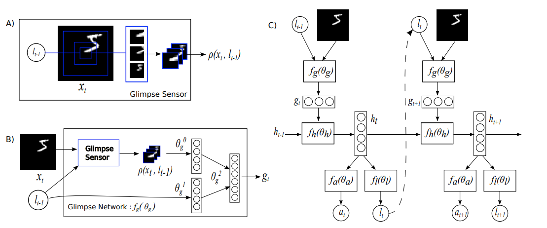
Retina Module #

This module is used to sample the input image. Given coordinates within the input image this module will take samples centered on the provided coordinates. The location coordinates used by the model are a pair of normalized (x,y) coordinates in the range of [-1,1].

The hyperparameters for the Retina module are the image size, the glimpse size and the number of scaled samples to capture for each glimpse. In the following illustration you can see that there are 3 samples each at a different scale and all centered on the same location within the input image. In the game of Catch, I've used an input image size of 24x24 pixels (the entire game is rendered on to a surface of this size) and a glimpse size of 6x6 pixels at three different scales. The scales are powers of two which gives us the following samples.

2^0 * 6 = 1 * 6 = 6; 6x6 pixel sample not downsampled
2^1 * 6 = 2 * 6 = 12; 12x12 pixel sample downsampled to 6x6 pixels
2^2 * 6 = 4 * 6 = 24; 24x24 pixel sample downsampled to 6x6 pixels

This is illustrated below:

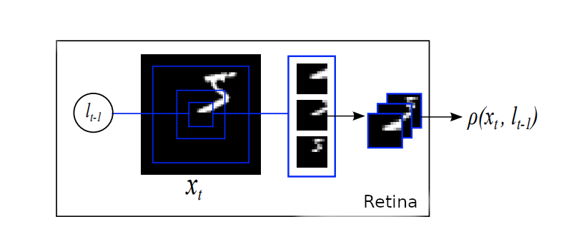
You can also see this in the first video in this article. The red,green,blue color-coded boxes show the samples taken at different scales. The "Individual Glimpses" show the 6x6 pixel downsampled data that is made available to the model. The model is not able to see any more of the input image other than these three 6x6 pixel samples.

An analogy to the very low resolution outer-most sample would be our peripheral vision.

Glimpse Module #

The Glimpse module is a simple network consisting of linear layers. One linear layer builds a set of features based on the input of the Retina module (Called "Glimpse Sensor" in the diagrams) described above. Another linear layer takes in the location of the retinal sensor for context. And a third linear layer integrates the two feature vectors together.

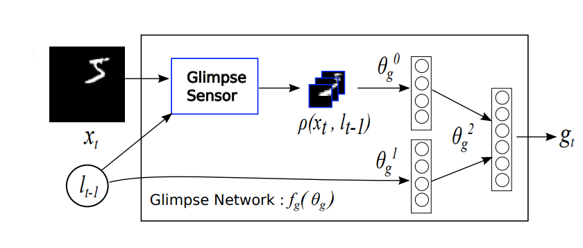
The output vector from the glimpse module is shown as g_t in the diagrams.

Core Module #

Since we have to be able to integrate features together across different samples over time, we need a recurrent core that can transfer hidden state across time steps. A recurrent model is basically a neural network with loops. In addition to the bottoms-up input, a recurrent model takes an additional input from itself generated at a previous timestep. For the game of catch, we use Long short-term memory, LSTM modules. The following diagram shows the data flow between two timesteps t(n) on the left and t(n+1) on the right.

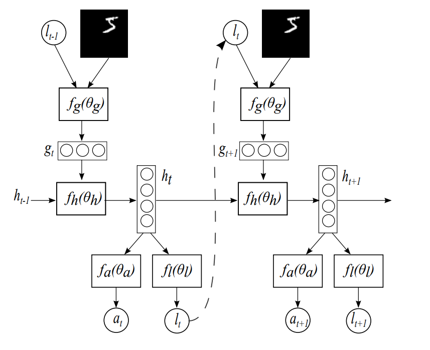
The output vector from the core module is shown as h_t in the diagrams.

Location Module #

Given the feature vectors that are generated by the recurrent Core module described above, the model has a simple linear layer that learns to generate the location to look at for the next time step. You can see this location being propogated to the next time step via the dashed-line in the prior diagram.

The output vector from the location module is shown as I_t in the diagrams.

Action Module #

Similar to the Location module described above. The Action module consists of a single linear layer that takes as input the feature vector from the recurrent Core module described above and generates an output action from the network.

For the game Catch, the network is exposed to every frame of gameplay and at each timestep, the action generated from this module is used to determine whether to move the paddle left or right.

In the case of MNIST classification, the network gets to make a configured number of "retinal fixations", the action generated from this module is ignored until the final fixation and that action is then used to determine the classification of the MNIST digit (0 through 9).

The output vector from the action module is shown as a_t in the diagrams.

Training #

The training consists of rolling out the policy currently encoded into the model's weights and measuring how well it does against the objective encoded in the loss function. It's important to have enough samples in each training step to ensure that we're evaluating the current policy accurately. A baseline (or target reward) is updated at each training step. The intent of this baseline is to bifurcate the actions that led to the most reward away from the actions that led to the least reward within the current training epoch. The model weights are then updated to encourage the best actions and to discourage the worst actions.

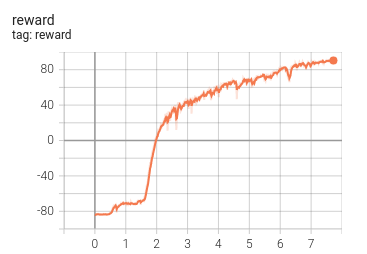
The catch model was able to get to a 90% success rate after about 7 hours of training.

tensorboard graph showing reward progress during training of Catch

Results #

The code I've provided in my repo was able to successfully reproduce all of the experiments described in the paper with the same or better performance.

Here are a few videos demonstrating the MNIST classification task as well.

mnist classification using the centered dataset

mnist classification using the translated dataset

Closing Thoughts #

Even though the problems described in this article are in the class of toy problems. I see them as a way to explore how the brain might be solving similar problems. Some other possible ideas for future exploration:

• One thing that I'd like to try would be to attempt full scene reconstruction for video with a recurrent network and a moveable limited-bandwidth sensor. If applied to a remote camera scenario this would have the potential of greatly reducing the amount of required upstream bandwidth and would allow more processing to be offloaded to the edge. For real world scenes, this would require that the model not only generate static pixels but would likely need to capture optical flow or even "object flow" to compensate for the lack of sensory input.

• One other big unsolved problem in machine learning is the hierarchical or part-wise decomposition of objects. The ability for the brain to model the world using reference frames is generally accepted as a key requirement for reasoning about the world and navigating it. It would be interesting to explore whether the concept of "hard attention" lends itself to models that maintain a current reference frame and learn to recursively model the world in this way.

I have some other ideas too, but would love to hear other ideas if you have them, so please share...

• Next: UFO Lands on Highway! Or Depth Estimation using ML
• Previous: Pong From Pixels.